Particle in a Box Lab

Question 1: Standing Waves
From your study of mechanical waves, what is the longest wavelength standing wave on a string of length L?


A:  The longest wavelength would be 2L.


Question 2: The de Broglie Relation
What is the momentum of the longest wavelength standing wave in a box of length L?


A:  Using de Broglie's equation p=h/2L.

Question 3: Ground State Energy
Assuming the particle is not traveling at relativistic speeds, determine an expression for the ground state energy.

Check your result by displaying the ground state energy.

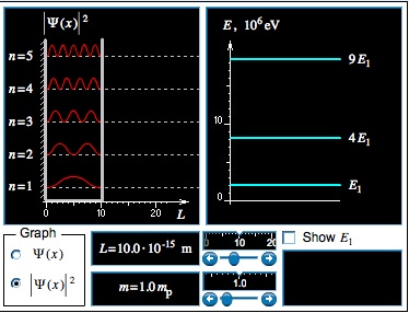
A:  E= (h^2)/8mL

Question 4: Increasing L
If the size of the box is increased, will the ground state energy increase or decrease?

A:  As the size of the box increases the ground state energy decreases.

Question 5: The Correspondence Principle: Large Size
In the limit of a very large box, what will happen to the ground state energy and the spacing between allowed energy levels? Can this result explain why quantum effects are not noticable in everyday, macroscopic situations?

A:  As the ground state energy gets smaller the spacing becomes continuous.

Question 6: The Correspondence Principle: Large Mass
In the limit of a very massive particle, what will happen to the ground state energy and the spacing between allowed energy levels?

A:  With and increase in the mass we have a decrease in ground state energies.

Question 7: Ground State Probability
If a measurement is made of the particle's position while in the ground state, at what position is it most likely to be detected?

A:  At its ground state a particle is most likely to be in the center.

Question 8: Probability: Dependence on Mass and Size
The most likely position to detect the particle, when it is in the ground state, is in the center of the box. Does this observation depend on either the mass of the particle or the size of the box?


A:  No, if the mass of the particle or the size of the box increase in the ground state energy the electron is still most likely to be found in the center.


Question 9: Probability: Dependence on Energy Level
The most likely position to detect the particle, when it is in the ground state, is in the center of the box. Does this observation hold true at higher energy levels?


A:  Yes even if energy levels are higher the particle is still most likely in the center of the box.


Question 10: The Correspondence Principle: Large n
In the limit of large n, what will happen to the spacing between regions of high and low probability of detection? Does this agree with what is observed in everyday, macroscopic situations?


A:  At a high n the spacing between the nodes gets closer and closer tell the energy becomes continuous.

Wave Packet Programming Lab

4 Sinusoid graph:

---------------------------------------------

from pylab import *

#Define constantsConstants

A=1 #Define the ampletude of the sin function

w=1 #sets the frequancey coefficient

#Calculation Loop: Note Nesting Carfully

for i in range(1,4):

    x = []

    sin_list = []

    for t in arange (-3.14, 3.14, 0.01):

        sine= A*sin(i*w*t)

        sin_list.append(sine)

        x.append(t)

    plot (x,sin_list)

show()

---------------------------------------

50 sinusoid graph:

--------------------------------------

from pylab import *

#Define constantsConstants

A=1 #Define the ampletude of the sin function

w=1 #sets the frequancey coefficient

#Calculation Loop: Note Nesting Carfully

for i in range(1,50):#every time the loop repeats this will change the harmonic

    x = [] # plots from -pi to +pi

    sin_list = [] #this includes the sine functions

    for t in arange (-3.14, 3.14, 0.01): # create tsh range of the graph and incriments

        sine= A*sin(i*w*t) #the function to be plotted

        sin_list.append(sine) # Adds the calculated vale from the sine function to the list appendex

        x.append(t)

    plot (x,sin_list)# plots values

show() #show the plot

----------------------------------------

Localized particle

---------------------------------------

from pylab import *

#Define constantsConstants

A=1 #Define the ampletude of the sin function

w=1 #sets the frequancey coefficient

Fourier_Series=[] #initialize the list of sine functions

#Calculate the harmonics of the sine functions

for i in range(1,300):#every time the loop repeats this will change the harmonic

    x = [] # plots from -pi to +pi

    sin_list = [] #this includes the sine functions

    for t in arange (-3.14, 3.14, 0.01): # create tsh range of the graph and incriments

        sine= A*sin(i*w*t) #the function to be plotted

        sin_list.append(sine) # Adds the calculated vale from the sine function to the list appendex

        x.append(t)

    #plot (x,sin_list)# plots values

    Fourier_Series.append(sin_list)

superposition = zeros(len(sin_list))

for function in Fourier_Series:

    for i in range(len(function)):

        superposition[i]+=function[i]

    

plot(x,superposition)

show()

--------------------------------------------

Envelope

-------------------------------------------

from pylab import *

#Define constantsConstants

A_list=[] #Define the amplitude of the sin function

w=1 #sets the frequancey coefficient

Fourier_Series=[] #initialize the list of sine functions

sigma = 1

coeff = 1

numberofharmonics=50

center = numberofharmonics/2

#Calculate the harmonics of the sine functions

for i in range(1,50):#every time the loop repeats this will change the harmonic

    x = [] # plots from -pi to +pi

    gauss = coeff*exp(-(i-center)**2/(2.*sigma**2))

    

    sin_list = [] #this includes the sine functions

    for t in arange (-3.14, 3.14, 0.01): # create tsh range of the graph and incriments

        sine= gauss*sin(i*w*t) #the function to be plotted

        sin_list.append(sine) # Adds the calculated vale from the sine function to the list appendex

        x.append(t)

    #plot(x,sin_list)# plots values

#show()

    Fourier_Series.append(sin_list)

superposition = zeros(len(sin_list))

for function in Fourier_Series:

    for i in range(len(function)):

        superposition[i]+=function[i]

plot(x,superposition)

show()

---------------------------------------------------

Wave packet

---------------------------------------------------

from pylab import *

#Define constantsConstants

w=1 #sets the frequancey coefficient

Fourier_Series=[] #initialize the list of sine functions

sigma = 10

coeff = 1

numberofharmonics=50

center = numberofharmonics/2

#Calculate the harmonics of the sine functions

for i in range(1,50):#every time the loop repeats this will change the harmonic

    x = [] # plots from -pi to +pi

    gauss = coeff*exp(-(i-center)**2/(2.*sigma**2))#Define the amplitude of the sin function

    sin_list = [] #this includes the sine functions

    for t in arange (-3.14, 3.14, 0.01): # create tsh range of the graph and incriments

        sine= gauss*sin(i*w*t) #the function to be plotted

        sin_list.append(sine) # Adds the calculated vale from the sine function to the list appendex

        x.append(t)

    #plot(x,sin_list)# plots values

#show()

    Fourier_Series.append(sin_list)

superposition = zeros(len(sin_list))

for function in Fourier_Series:

    for i in range(len(function)):

        superposition[i]+=function[i]

plot(x,superposition)

show()

--------------------------------------------------

Relativity Lab

Relativity of Time:

Question 1: Distance traveled by the light pulse
How does the distance traveled by the light pulse on the moving light clock compare to the distance traveled by the light pulse on the stationary light clock?


A:  The light on the moving light clock must travel a greater distance than the light on the stationary light clock.  Although they both go up and down, the moving light clock has a component vt in the direction of motion that must be factored in.


Question 2: Time interval required for light pulse travel, as measured on the earth
Given that the speed of the light pulse is independent of the speed of the light clock, how does the time interval for the light pulse to travel to the top mirror and back on the moving light clock compare to on the stationary light clock?


A:  From the stationary observer it appears as though the light takes longer to complete a cycle due to the fact that it has a larger distance to travel.


Question 3: Time interval required for light pulse travel, as measured on the light clock
Imagine yourself riding on the light clock. In your frame of reference, does the light pulse travel a larger distance when the clock is moving, and hence require a larger time interval to complete a single round trip?


A:  From the point of view of the moving observer the time taken for the journey is the same as if the light clock were stationary, this is due to the fact that from the moving observes point of view there is actually no extra distance traveled and the light appears to only go up and down the y axis.


Question 4: The effect of velocity on time dilation
Will the difference in light pulse travel time between the earth's timers and the light clock's timers increase, decrease, or stay the same as the velocity of the light clock is decreased?


A:  The faster the light clock moves the greater the difference between it and the stationary clock.


Question 5: The time dilation formula
Using the time dilation formula, predict how long it will take for the light pulse to travel back and forth between mirrors, as measured by an earth-bound observer, when the light clock has a Lorentz factor (γ) of 1.2.


A:  (1.2)(6.67E-6)= 8E-6 s


Question 6: The time dilation formula, one more time
If the time interval between departure and return of the light pulse is measured to be 7.45 µs by an earth-bound observer, what is the Lorentz factor of the light clock as it moves relative to the earth?


A: (7.45E-6)/(6.67E-6)=1.12

Relativity of Length:


Question 1: Round-trip time interval, as measured on the light clock
Imagine riding on the left end of the light clock. A pulse of light departs the left end, travels to the right end, reflects, and returns to the left end of the light clock. Does your measurement of this round-trip time interval depend on whether the light clock is moving or stationary relative to the earth?


A:  It does matter as if the light clock is moving it will take longer for the light to travel to the right end a very short time to return, this will make the total trip time seem longer.


Question 2: Round-trip time interval, as measured on the earth
Will the round-trip time interval for the light pulse as measured on the earth be longer, shorter, or the same as the time interval measured on the light clock?


A:  it will seem longer for reasons mentioned above.


Question 3: Why does the moving light clock shrink?
You have probably noticed that the length of the moving light clock is smaller than the length of the stationary light clock. Could the round-trip time interval as measured on the earth be equal to the product of the Lorentz factor and the proper time interval if the moving light clock were the same size as the stationary light clock?


A:  If the moving clock were the same size as the stationary clock then the Lorentz factor would not be valid.  The moving clock must shrink to uphold the Lorentz factor.


Question 4: The length contraction formula
A light clock is 1000 m long when measured at rest. How long would earth-bound observer's measure the clock to be if it had a Lorentz factor of 1.3 relative to the earth?


A: (1000)/1.3= 769 m