Python Tutorial

from visual.graph import *

#define values
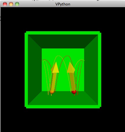
ball = sphere(pos=(-5,2,-1), radius=.5, color=color.red)
ball2= sphere(pos=(5,2,-1), radius=.5, color=color.orange)
wallR = box(pos=(6,0,0), size=(.5,12,12), color=color.green)
wallL = box(pos=(-6,0,0), size=(.5,12,12), color=color.green)
wallF = box(pos=(0,0,-6), size=(12,12,.5), color=color.green)
wallT = box(pos=(0,6,0), size=(12,.5,12), color=color.green)
wallB = box(pos=(0,-6,0), size=(12,.5,12), color=color.green)
dt = 0.02


ball.velocity = vector(2,3,-5)
ball.trail = curve(color=ball.color)
bv = arrow(pos = ball.pos, axis = ball.velocity, color=color.yellow)

ball2.velocity = vector(-2,3,-5)
ball2.trail = curve(color=ball2.color)
bv2 = arrow(pos = ball2.pos, axis = ball2.velocity, color=color.yellow)

while(1==1):
    rate(50)
 
  
    ball.acceleration = vector(0,-9.81,0)
    ball.pos = ball.pos + ball.velocity*dt + .5*ball.acceleration*dt*dt
    ball.velocity = ball.velocity + ball.acceleration*dt

    ball2.acceleration = vector(0,-9.81,0)
    ball2.pos = ball2.pos + ball2.velocity*dt + .5*ball2.acceleration*dt*dt
    ball2.velocity = ball2.velocity + ball2.acceleration*dt

    if ball.x >= (wallR.x - .75):
        ball.velocity.x = -ball.velocity.x
    if ball.x <= (wallL.x + .75):
        ball.velocity.x = -ball.velocity.x
    if ball.y >= (wallT.y - .75):
        ball.velocity.y = -ball.velocity.y
    if ball.y <= (wallB.y + .75):
        ball.velocity.y = -ball.velocity.y
    if ball.z <= (wallF.z +.75):
        ball.velocity.z = -ball.velocity.z
    if ball.z >= 5.5:
        ball.velocity.z = -ball.velocity.z

    if ball2.x >= (wallR.x - .75):
        ball2.velocity.x = -ball2.velocity.x
    if ball2.x <= (wallL.x + .75):
        ball2.velocity.x = -ball2.velocity.x
    if ball2.y >= (wallT.y - .75):
        ball2.velocity.y = -ball2.velocity.y
    if ball2.y <= (wallB.y + .75):
        ball2.velocity.y = -ball2.velocity.y
    if ball2.z <= (wallF.z +.75):
        ball2.velocity.z = -ball2.velocity.z
    if ball2.z >= 5.5:
        ball2.velocity.z = -ball2.velocity.z

    if ball.pos.x == ball2.pos.x:
        ball.velocity.x= -ball.velocity.x
        ball2.velocity.x= -ball2.velocity.x
  
      
    bv.pos = ball.pos
    bv.axis = ball.velocity/2
    ball.trail.append(pos = ball.pos)
    bv2.pos = ball2.pos
    bv2.axis = ball2.velocity/2
    ball2.trail.append(pos = ball2.pos)
  
------------------------------------------------------------------

Diffraction Lab

Purpose:

The purpose of this lab was to test the diffraction of light against a compact disc.  A compact disc contains information by having small burns on the disk, these burns can be viewed by shining a lazar light onto the CD.  The equation used was:

y=mLR/2d

where y is distance from central maxima, m is number of minima, L is wavelength, R is distance from diffraction gradient, and d is distance between gratings which is our target variable in this experiment.

Method:

The experiment was assembled by using a standard compact disc and a laser with a wavelength of 670 nm +/- 20 nm.  Two sets of data were taken.  The first was at a distance of 2.00 m +/- .15 m.  At this distance the maxima were measured on the right of the central maxima and on the left of the central maxima.  To our surprise the two sides were different and one of the sides was also noted to be curved.  both sides were measured and charted.

	right (cm)	left (cm)	average (cm)	Uncertanty (cm)
m1	2.12	3.10	2.61	0.98
m2	4.70	5.50	5.10	0.80
m3	6.80	8.60	7.70	1.80
m4	8.60	11.10	9.85	2.50
m5	10.40	14.40	12.40	4.00

The varying values leads to a high uncertainty and makes the data less useful than desired.  Next we set up the experiment in a different way.  We place a white board close to the CD and place the Laser close to the CD as well.  By lowering the distance from grating to diffraction pattern we reduced the uncertainty of the data.  With a new R= 0.07 m +/- 0.015 m we got consistent data on both sides of the central maxima

	average (cm)	Uncertanty (cm)
m1	2.80	0.20
m2	4.20	0.40

Using our equation for diffraction grating we determined a value of d= 977.1 nm +/- 279.5 nm

Conclusion:

The value obtained for the distance between gratings was 977.1 nm +/- 279.5 nm.  The actual known value of the distance is around 1600 nm which is out of our uncertainty range and has an error percent of  21.5% from the furthest reaches of our uncertainty.  Although the data is on the same order of magnitude when uncertainty is taken into account, the actual results are not accurate at all.  Results may have been off due to having R be to small, if slightly larger measurements of minima distances would have been easier to get.

Measuring Thickness of Human Hair Using Young's Method

Purpose:

This experiment was a recreation of the famous Young’s double slit experiment originally carried out in 1800 by Thomas Young.  The slight variation on the experiment was that a hair was used as the divider of the light source.  This added an additional easement to the experiment that gave it a bit more depth.  When the light was projected on a whiteboard an interference pattern was viewed, confirmation of lights wave like properties.  This pattern was measured in an attempt to confirm the Young’s double slit equation.

Method and Results:

A hear was plucked from one of the members of the lab group and this hear was measured for its thickness (d).  Next the hair was taped to the hole of an index card in such a manner that divided the hole punched circle evenly.  This card was set in place and a laser of known pre measured wavelength was focused through the hole.  A white board was placed at varying distances to easily view the interference pattern.  The distance from the index card to the board was measured (R).  Next the interference pattern was measure from 4 interference fringes (y).  These values were then used to confirm the thickness of the hair measured with the micrometer.

Trial	R (m)	y (m)	M
1	2.00	0.0765	4
2	1.68	0.0630	4
3	3.62	0.1100	4

Wavelength:  670 nm +/- 20 nm

Measured Thickness of hair:  0.0245 mm+/- 0.0015 mm

Calculated thickness:

Trial 1: 0.0701 mm +/-  0.0030 mm

Trial 2: 0.0715 mm +/-  0.0030 mm

Trial 3: 0.0882 mm +/-  0.0030 mm

            Average: 0.0766 mm +/- 0.0090 mm

Conclusion:

The thickness measured with the Young’s double slit experiment gave precise results and two of the three trials were within the measured uncertainty.  These values seem much more reliable than the micrometer measurement as most groups were having trouble getting measurements from the equipment.  This coupled with the precision of the Young’s method leads me to believe the diameter of the hair is the average of the Young’s result.

Real Image through a Lens Lab

Purpose:

The purpose of this lab was to explore the actions of light as it moves through a lens.  A light source was used to project a real image through a magnifying glass and on to a white board to view how the light was refracted and altered.

Method and Results:

A magnifying glass was chosen and this glass was measured for its focal point.  The method for the measurement was to use the suns light to focus a light rays onto the ground.  Due to the magnifying glass being a convex lens it is know that the point at which the light is focused through it from a far off object is at the focal point.  Three measurements were taken from the focal point on the ground to the lens.  These measurements were taken for an average and to determine the uncertainty of the method.

f1= 14.10 cm
f2= 15.80 cm
f3= 15.00 cm
favg= 14.97 cm +/- 1.70 cm

The magnifying glass was set up distances from the light source of known multiples of the average focal length.  A white board was placed behind the lens and adjusted in tell the image was focused.  The distance from the lens to the white board was measured as was the height of the real image.

Relative to f	Object distance (cm)	Image distance (cm)	Object height (cm)	Image height (cm)	M	Type of image
5f	74.85	23.5	3	1.30	0.433	inverted/reversed
4f	59.88	24.5	3	1.75	0.5833	inverted/reversed
3f	44.91	28.7	3	1.95	0.65	inverted/reversed
2f	29.94	44.5	3	5.20	1.733	inverted/reversed
1.5f	22.46	332.5	3	53.60	17.867	inverted/reversed

A measurement was taken at distance 0.5f but the image could not be focused.  The object and image distance were graphed and an inverse relationship was found.

The inverse of both values was then taken and a linear relationship was discovered.

Conclusion:


The absolute value of the slope of the graph is 0.7738 which is a value that is off from the expected value of one as this is the value of n in air.  this discrepancy could be explained by the large uncertainty involved in our measurement of the focal point as the uncertainty of 1.70 cm is a large value.  More likely though the % error of 22.6% is due to the low number of points measured and the arbitrary nature in which the focused real image was obtained.  These cupeled with the fact that there was not an adequate light experiment setup lead to much uncertainty.  

Concave Convex Mirrors

Purpose:

The Purpose of this experiment was to explore the image formed by both a convex and concave mirror.  Concave and convex mirrors are both considered spherical mirrors and both behave differently than a traditional plane mirror.  One of the most apparent differences is in the distortion of the height and distance of the image.

Method and Results:

Objects were held in from of both a concave and convex mirror at separate times.  The object was moved in front of the mirror and inspected at different distances and orientations.  Next ray diagrams were constructed form each of the mirrors.

Convex Mirror

With the convex mirror the focal point is located on the inside of the mirror and this is on the opposite side of the reflected light rays.  This leads for the image to be on the inside of the mirror leading to a virtual image.  The closer the object is to the mirror the larger the image will be to the extent that if the image is close to the mirror the image will be larger than the image.

S= 6.20 cm               s= 1.95 cm
H= 3.10 cm              h= 0.75 cm

Concave Mirror

With a concave mirror the results are different.  The main result is that the image is on the same side as the outgoing rays making them a real image.  This image is inverted so long as the distance of the object is grater than the focal point which in this type of mirror is located on the same side as the object.  

S= 2.50 cm                                s= 0.75 cm
H= 11.40 cm                             h= 3.30 cm

Conclusion:

In conclusion the behavior of light rays in spherical mirrors is much different than in plane mirrors.  The image can be virtual or real.  The image can be erect or inverted.  The height of the object can vary drastically.  a majority of these differences occur due to the addition of the center of curvature which in a plane mirror goes to infinity and is no longer important leading to a simplified equation for light ray behavior.